Mastering Excel: Switching from VLOOKUP to INDEX-MATCH – 2024

Mastering Excel: Switching from VLOOKUP to INDEX-MATCH

VLOOKUP is a popular Excel function for looking up values in a table, but it has limitations. INDEX and MATCH, when used together, offer a more flexible and powerful alternative. This comprehensive guide will walk you through the process of replacing VLOOKUP with INDEX/MATCH, empowering you with greater control and efficiency in your data analysis.

Why Replace VLOOKUP with INDEX/MATCH?

• Flexibility: INDEX/MATCH can look up values to the left, unlike VLOOKUP, which is restricted to rightward lookups.
• Efficiency: INDEX/MATCH can be faster than VLOOKUP, especially with large datasets.
• Dynamic Column References: Easily adjust the return column without manually changing the formula.
• Error Handling: INDEX/MATCH can gracefully handle errors if a lookup value is not found.

Understanding INDEX/MATCH

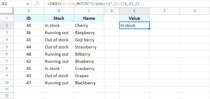
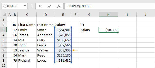
• INDEX: Returns a value from a table or range based on its row and column numbers.
• MATCH: Returns the relative position of an item in a range that matches a specified value.

By combining these functions, you can create a powerful lookup formula that overcomes the limitations of VLOOKUP.

How to Replace VLOOKUP with INDEX/MATCH

1. Identify Lookup Value and Table Array:

   • Determine the value you want to look up (lookup_value) and the table or range where the data resides (table_array).

2. Find the Lookup Column:

   • Identify the column in the table_array where the lookup_value is located (lookup_column).

3. Find the Return Column:

   • Identify the column in the table_array where the value you want to return is located (return_column).

4. Construct the Formula:

   • Use the MATCH function to find the row number of the lookup_value in the lookup_column:
     • MATCH(lookup_value, lookup_column, 0) (0 for exact match)
   • Use the INDEX function to retrieve the value from the return_column in the row found by MATCH:
     • INDEX(return_column, MATCH(lookup_value, lookup_column, 0))

Example

Let’s say you have a table with product names in column A and prices in column B. You want to find the price of a specific product (e.g., “Product A”).

1. Lookup Value: “Product A”
2. Table Array: A1:B5
3. Lookup Column: A1:A5
4. Return Column: B1:B5

The INDEX/MATCH formula would be:

=INDEX(B1:B5, MATCH("Product A", A1:A5, 0))

Additional Tips

• Error Handling: Use the IFERROR function to handle cases where the lookup_value is not found:
  • =IFERROR(INDEX(return_column, MATCH(lookup_value, lookup_column, 0)), "Not Found")
• Approximate Matches: For approximate matches, use 1 or -1 as the match_type in the MATCH function.
• Multiple Criteria: Combine INDEX/MATCH with other functions like IF or AND to perform lookups based on multiple criteria.

Conclusion

By mastering INDEX/MATCH, you can overcome the limitations of VLOOKUP and unlock a new level of flexibility and power in your Excel data analysis. This versatile combination of functions allows you to perform lookups in any direction, handle errors gracefully, and create more dynamic and efficient spreadsheets.

Related articles

» How to Limit Rows and Columns in an Excel Worksheet
» Troubleshooting “OLE Action Excel” Error in Microsoft Excel
» Ways To Alternate Row Colors in Excel [Guide/]