Excel Conditional Formatting Made Simple: A Beginner’s Guide

Excel’s conditional formatting is a powerful tool that allows you to dynamically change the appearance of cells based on specific criteria. Whether you want to highlight top performers, flag deadlines, or visualize data trends, conditional formatting can transform your spreadsheets into insightful dashboards. This tutorial will guide you through the basics and advanced techniques of conditional formatting, empowering you to unlock the full potential of your data.
Why Use Conditional Formatting?
Before we dive into the how-to, let’s explore the benefits of conditional formatting:
- Enhanced Data Visualization: Quickly identify patterns, outliers, and trends in your data.
- Improved Readability: Make your spreadsheets easier to understand and interpret.
- Automated Formatting: Save time by automatically applying formatting based on rules.
- Data Validation: Highlight errors or inconsistencies in your data.
Getting Started with Conditional Formatting

- Select Your Data: Highlight the cells, range, or entire table you want to apply formatting to.
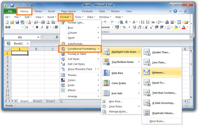
- Access Conditional Formatting: Go to the “Home” tab in the Excel ribbon and click on “Conditional Formatting.”
- Choose a Rule Type: Excel offers various rule types, such as:
- Highlight Cells Rules: Highlight cells based on their values (e.g., greater than, less than, between).
- Top/Bottom Rules: Highlight the top or bottom values in a range.
- Data Bars, Color Scales, Icon Sets: Visually represent values using bars, color gradients, or icons.
- New Rule: Create custom rules using formulas or specific criteria.
- Configure Your Rule: Select the rule type and customize the criteria and formatting options.
- Apply: Click “OK” to apply the conditional formatting.
Advanced Conditional Formatting Techniques

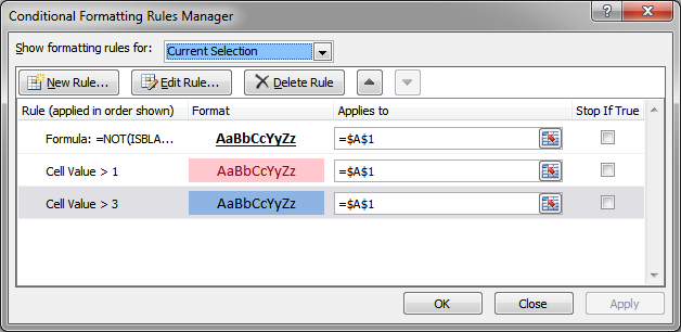
- Multiple Rules: You can apply multiple conditional formatting rules to the same cells. Excel evaluates the rules in order and applies the first rule that matches.
- Formula-Based Rules: Use formulas to create complex conditional formatting rules based on calculations or comparisons.
- Stop If True: Prevent subsequent rules from being evaluated if a previous rule is true.
- Manage Rules: View, edit, or delete existing rules using the “Conditional Formatting Rules Manager.”
Examples of Conditional Formatting in Action
- Highlighting Due Dates: Use a rule to highlight cells containing dates that are approaching or past due.
- Grading Students: Apply color scales to visualize student grades, with higher grades getting greener and lower grades getting redder.
- Tracking Inventory: Use icon sets to indicate stock levels (e.g., green checkmark for in stock, red X for out of stock).
- Analyzing Sales Data: Apply data bars to sales figures to quickly identify top-performing products or regions.
Tips for Effective Conditional Formatting
- Keep It Simple: Avoid using too many rules or overly complex formatting, as it can make your spreadsheet difficult to read.
- Test Your Rules: Always test your conditional formatting rules to ensure they are working as expected.
- Use Meaningful Colors: Choose colors that are intuitive and convey the meaning of your data.
- Consider Your Audience: Tailor your conditional formatting to the needs and preferences of your audience.
Conclusion
By mastering Excel conditional formatting, you can transform your spreadsheets into powerful tools for data analysis, visualization, and communication. Experiment with different rule types and formatting options to discover the endless possibilities this feature offers. With practice and creativity, you’ll be able to create stunning and informative spreadsheets that impress your colleagues and clients.
Related articles
» How to Use Conditional Formatting to Make Your Excel Data Stand Out
»How to insert page break in Excel worksheet
»Expense Record & Tracking Sheet Templates for Excel
»How to Calculate CAGR in Excel

