How to Modify Legends in Excel – 2024

How to Modify Legends in Excel

Legends are essential components of charts in Microsoft Excel, providing clarity and context by labeling the different data series. Editing legends allows you to customize their appearance, position, and content to best suit your needs. This guide will walk you through the various ways to edit legends in Excel, ensuring your charts are informative and visually appealing.

1. Adding and Removing Legend Entries

• Add a Legend Entry:

  1. Click on your chart to select it.
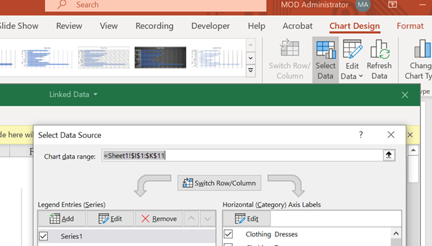
  2. Go to the “Chart Design” tab and click “Select Data.”
  3. In the “Select Data Source” dialog box, click “Add” under “Legend Entries (Series).”
  4. Enter the series name and values, then click “OK.”

• Remove a Legend Entry:

  1. Click on your chart to select it.
  2. Click the legend to select it.
  3. Right-click on the legend entry you want to remove and select “Delete.”

2. Changing Legend Position

• Predefined Positions:

  1. Click on your chart to select it.
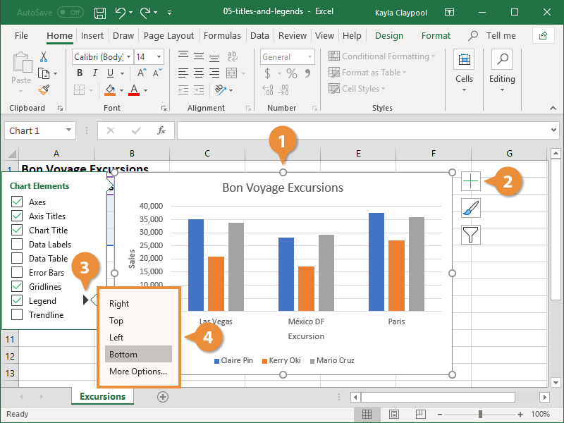
  2. Click the “+” icon next to the chart (Chart Elements button).
  3. Check the “Legend” box.
  4. Click the arrow next to “Legend” and choose a position (right, top, left, bottom).

• Custom Position:

  1. Click on the legend to select it.
  2. Drag the legend to your desired location within the chart area.

3. Editing Legend Text

• Change Legend Entry Name:

  1. Click on your chart to select it.
  2. Click the legend to select it.
  3. Double-click the legend entry you want to edit.
  4. In the “Format Legend Entry” dialog box, modify the text in the “Series name” field.
  5. Click “OK.”

• Change Font, Size, and Color:

  1. Click on the legend to select it.
  2. Use the formatting options in the “Home” tab (font, size, color, etc.) to customize the legend text.

4. Formatting the Legend Box

• Border, Fill, and Effects:
  1. Click on the legend to select it.
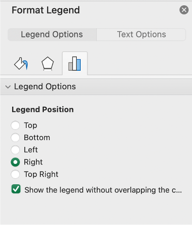
  2. Right-click and select “Format Legend.”
  3. In the “Format Legend” pane, adjust the border style, fill color, and apply effects like shadow or glow.

5. Adding a Legend Without a Chart

• You can create a legend without an accompanying chart using text boxes and shapes.
• Steps:
  1. Insert text boxes to represent legend entries.
  2. Insert shapes (e.g., squares, circles) to represent the data series colors or patterns.
  3. Arrange the text boxes and shapes to create your legend.
  4. Group the elements to move and resize them together.

Tips and Tricks:

• Show/Hide Legend: To show or hide the legend, click the “+” icon next to the chart and check/uncheck the “Legend” box.
• Legend Key: The legend key is the small colored square or symbol that represents a data series in the legend. You can customize its size and shape in the “Format Legend” pane.
• Linked to Data: If you change the data in your chart, the legend will automatically update to reflect the changes.

By following these steps and utilizing the various editing options, you can create clear, informative, and visually appealing legends for your Excel charts.