Essential Excel Formulas: 10 Critical Functions for Mastering Data Analysis

Excel is a powerhouse for data analysis and manipulation, and its vast array of functions can be overwhelming. However, mastering a few essential formulas can significantly enhance your productivity and unlock the true potential of your spreadsheets. This comprehensive guide will introduce you to the top 10 Excel functions that every data enthusiast should know.
1. SUM:

- Purpose: Calculates the total of a range of numbers.
- Syntax:
=SUM(number1, [number2], ...) - Example:
=SUM(A1:A10)adds up the values in cells A1 through A10.
2. AVERAGE:

- Purpose: Calculates the average (mean) of a range of numbers.
- Syntax:
=AVERAGE(number1, [number2], ...) - Example:
=AVERAGE(B1:B5)calculates the average of the values in cells B1 through B5.
3. COUNT:

- Purpose: Counts the number of cells containing numerical values in a range.
- Syntax:
=COUNT(value1, [value2], ...) - Example:
=COUNT(C1:C8)counts the number of cells with numerical values in cells C1 through C8.
4. IF:

- Purpose: Performs a logical test and returns one value if the test is TRUE and another value if the test is FALSE.
- Syntax:
=IF(logical_test, value_if_true, value_if_false) - Example:
=IF(D1>10, "Pass", "Fail")returns “Pass” if the value in cell D1 is greater than 10, and “Fail” otherwise.
5. VLOOKUP:

- Purpose: Searches for a value in the first column of a table and returns a corresponding value from another column in the same row.
- Syntax:
=VLOOKUP(lookup_value, table_array, col_index_num, [range_lookup]) - Example:
=VLOOKUP("Apple", A1:B5, 2, FALSE)searches for “Apple” in column A and returns the corresponding value from column B.
6. INDEX & MATCH:

- Purpose: A more flexible alternative to VLOOKUP that can search both vertically and horizontally.
- Syntax:
=INDEX(array, row_num, [col_num])and=MATCH(lookup_value, lookup_array, [match_type]) - Example:
=INDEX(B1:B5, MATCH("Apple", A1:A5, 0))achieves the same result as the VLOOKUP example above.
7. SUMIF:

- Purpose: Adds up the values in a range that meet a specified criterion.
- Syntax:
=SUMIF(range, criterion, [sum_range]) - Example:
=SUMIF(E1:E10, ">5")adds up the values in cells E1 through E10 that are greater than 5.
8. COUNTIF:

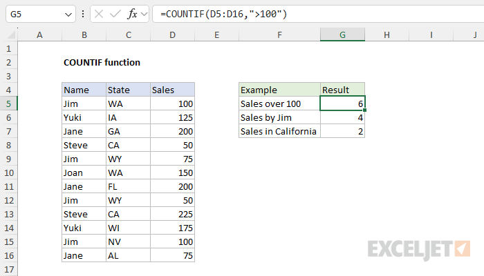
- Purpose: Counts the number of cells in a range that meet a specified criterion.
- Syntax:
=COUNTIF(range, criterion) - Example:
=COUNTIF(F1:F15, "Yes")counts the number of cells in cells F1 through F15 that contain “Yes.”
9. LEFT, RIGHT, MID:

- Purpose: Extract specific characters or substrings from text strings.
- Syntax:
=LEFT(text, num_chars)=RIGHT(text, num_chars)=MID(text, start_num, num_chars)
10. CONCATENATE:

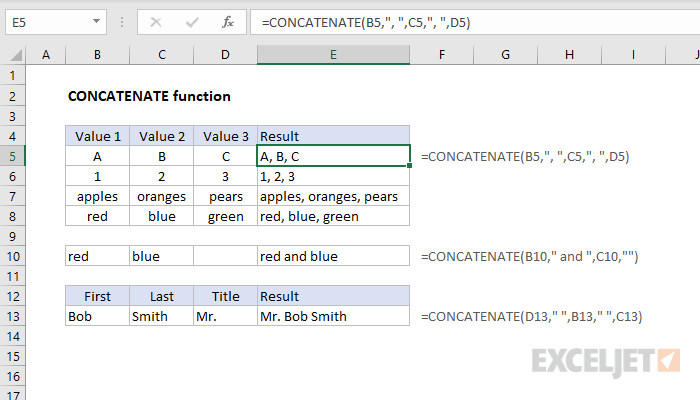
- Purpose: Combines text strings from multiple cells into one cell.
- Syntax:
=CONCATENATE(text1, [text2], ...) - Example:
=CONCATENATE(G1, " ", G2)combines the text in cells G1 and G2 with a space in between.
By mastering these essential Excel functions, you’ll be well on your way to becoming a data analysis pro. Remember, practice is key, so don’t hesitate to experiment with different formulas and scenarios. With time and dedication, you’ll be able to leverage the full power of Excel to gain valuable insights from your data.
Related Articles
» Excel Quick Analysis Tool: Streamline Data Analysis Effortlessly
» Creating a Data Entry Form in Excel: Simplify Your Data Input Process
» Create a Custom List in Excel | Step-by-Step Guide

