Excel VLOOKUP Mastery: A Comprehensive Step-by-Step Guide to Excel’s Most Powerful Function

Excel’s VLOOKUP function is one of the most powerful tools in data analysis and lookup operations. If you’re dealing with large datasets and need to find specific information from one table to another, VLOOKUP (Vertical Lookup) is essential. In this guide, we’ll break down VLOOKUP step by step, making it easy for anyone to use this incredible function effectively.
What is VLOOKUP?
VLOOKUP stands for “Vertical Lookup.” It allows you to search for a value in the leftmost column of a table and return a value in the same row from a specified column. For example, if you have a product list and want to find the price of a particular item based on its name, VLOOKUP will help you retrieve that information efficiently.
Syntax of VLOOKUP
Before diving into the step-by-step guide, let’s first understand the syntax of the VLOOKUP function:
=VLOOKUP(lookup_value, table_array, col_index_num, [range_lookup])
- lookup_value: The value you want to search for (e.g., a product name or ID).
- table_array: The range where the VLOOKUP will search (e.g., the table with your data).
- col_index_num: The column number in the table from which the matching value should be returned.
- [range_lookup]: A logical value (TRUE or FALSE) that specifies whether you need an exact or approximate match.
How to Use VLOOKUP: Step-by-Step
Step 1: Prepare Your Data
Ensure your data is properly organized. The column that contains the value you want to search should be the first (leftmost) column of the table. Other columns will contain the information you want to retrieve.
Example:

In this example, we have a table with Product IDs, Product Names, and Prices.
| Product ID | Product Name | Price |
|---|---|---|
| 101 | Apple | $1 |
| 102 | Banana | $0.5 |
| 103 | Orange | $0.8 |
Step 2: Insert the VLOOKUP Function
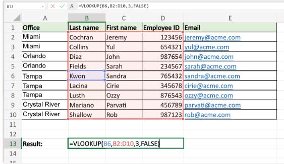
Click on the cell where you want the result to appear. Let’s say you want to find the price of a specific product using the Product Name.
- Select the empty cell and start typing the function:
php
=VLOOKUP("Banana", A2:C4, 3, FALSE)
- “Banana” is the value we are looking up.
- A2
is the range of the table.
- 3 refers to the third column (Price) from which we want to retrieve the result.
- FALSE ensures an exact match.
- Hit Enter. You’ll see the price of “Banana” ($0.5) returned in the cell.
Example:

Step 3: Lookup with a Cell Reference
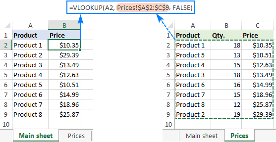
Instead of manually typing the value (e.g., “Banana”), you can use a cell reference to make your formula dynamic.
- Let’s assume you have “Banana” in cell E2. Modify your formula to:
php
=VLOOKUP(E2, A2:C4, 3, FALSE)
Now, anytime you change the value in E2, the formula will return the corresponding price from the table.
Example:

Range Lookup: Exact Match vs. Approximate Match
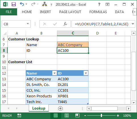
The [range_lookup] argument in VLOOKUP allows you to specify whether you want an exact match (FALSE) or an approximate match (TRUE).
Exact Match (FALSE)
This is the most common usage. When you need to find an exact value, you should set range_lookup to FALSE.
- For example, using the formula:
php
=VLOOKUP("Apple", A2:C4, 3, FALSE)
This will return the exact price for “Apple” ($1).
Approximate Match (TRUE)
If you’re working with a sorted list and want to find the closest match, you can use TRUE. This is helpful when searching for numbers in a range.
- For example:
php
=VLOOKUP(150, A2:B10, 2, TRUE)
This formula will look for the closest match to 150 in a sorted list.
Example:

Common Errors in VLOOKUP
- #N/A Error: Occurs when the function can’t find the lookup value. Ensure the value exists in the leftmost column of your table or check for spelling errors.
- #REF! Error: This happens when the col_index_num is larger than the number of columns in the table array.
- #VALUE! Error: This can occur if the table range isn’t correctly defined or if there’s an issue with the lookup value.
Tips and Tricks for Mastering VLOOKUP
- Use Named Ranges: Instead of manually selecting the table array, you can name your range. This will make your formulas more readable and easier to manage.
- Combine with IFERROR: Wrap VLOOKUP in an IFERROR function to handle errors gracefully:
less
=IFERROR(VLOOKUP(E2, A2:C4, 3, FALSE), "Not Found")
- Use INDEX-MATCH for More Flexibility: While VLOOKUP is powerful, it can only search left to right. For more flexibility (like searching in both directions), consider using the INDEX-MATCH combination.
Conclusion
The VLOOKUP function is a fundamental tool in Excel that can save you hours when working with large datasets. By mastering its syntax and learning a few tricks along the way, you can significantly improve your productivity and efficiency in handling data. Whether you need to lookup prices, names, or other types of information, VLOOKUP is a go-to function for Excel users of all levels.
