Step-by-Step Guide to Transposing Rows and Columns in Excel – 2024

Step-by-Step Guide to Transposing Rows and Columns in Excel

Switching rows and columns in Excel, also known as transposing data, is a useful technique when you need to reorient your data for better analysis or presentation. This feature allows you to flip your data set, converting rows into columns and vice versa. In this guide, we’ll walk you through the steps to transpose data in Excel, using both built-in tools and advanced techniques to help you manage your spreadsheets more effectively.

1. Why Switch Rows and Columns in Excel?

Switching rows and columns can enhance data presentation and make it easier to analyze specific information. Here are a few reasons why you might want to transpose your data:

• Improved Readability: Transposing data can make your table more readable, especially when dealing with a large number of columns or rows.
• Better Data Organization: Helps in reorganizing data to match specific requirements or formats.
• Enhanced Data Analysis: Facilitates easier comparison and analysis by changing the orientation of the data set.

Understanding these benefits helps you decide when transposing your data in Excel might be helpful.

2. How to Switch Rows and Columns Using the Transpose Feature

Excel offers a built-in “Transpose” feature that allows you to quickly switch rows and columns.

Step-by-Step Guide to Using the Transpose Feature:

1. Select the Data Range:
   • Highlight the data range you want to transpose. Make sure to include headers if they are part of your data.
2. Copy the Selected Data:
   • Right-click on the selected range and choose “Copy” from the context menu, or press Ctrl + C on your keyboard.
3. Choose the Destination for Transposed Data:
   • Click on the cell where you want the transposed data to start. Ensure there is enough space for the transposed data to avoid overwriting existing data.
4. Open the Paste Special Menu:
   • Right-click on the destination cell, choose “Paste Special…” from the context menu.
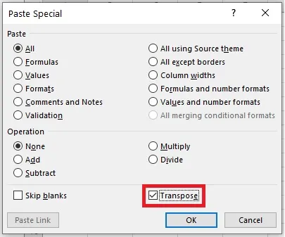
5. Select ‘Transpose’ Option:
   • In the “Paste Special” dialog box, check the “Transpose” option at the bottom.
6. Click ‘OK’ to Apply:
   • Click “OK” to apply the transpose function. Your data will be transposed, switching rows with columns.

3. Transposing Data Using the TRANSPOSE Function

For dynamic data that you might need to update frequently, using the TRANSPOSE function is more efficient. This function creates a dynamic array that updates automatically when the source data changes.

Step-by-Step Guide to Using the TRANSPOSE Function:

1. Select the Range for Transposed Data:
   • Click on the cell where you want to begin the transposed data. Select a range that matches the dimension of the original data (rows will become columns and vice versa).
2. Enter the TRANSPOSE Formula:
   • Type the formula =TRANSPOSE( and then select the range of the original data.

   Example Formula:

   If your original data is in cells A1:C3, the formula would be:

   $$=TRANSPOSE(A1:C3)$$
3. Press ‘Ctrl + Shift + Enter’:
   • Since TRANSPOSE is an array formula, you need to press Ctrl + Shift + Enter to execute it. Excel will automatically fill the selected range with the transposed data.
4. Dynamic Updates:
   • Any changes to the original data will automatically reflect in the transposed data because of the dynamic link created by the TRANSPOSE function.

4. Using Power Query to Transpose Data

Power Query, a powerful data transformation tool in Excel, provides another method to transpose data, particularly useful for larger or more complex data sets.

Step-by-Step Guide to Using Power Query:

1. Load Data into Power Query:
   • Select your data range, then go to the “Data” tab and choose “From Table/Range” to load your data into Power Query.
2. Open the Power Query Editor:
   • The Power Query Editor window will open, displaying your data.
3. Transpose the Data:
   • Click on the “Transform” tab in the Power Query Editor, then select “Transpose” to switch rows and columns.
4. Close and Load:
   • After transposing, click on “Close & Load” to load the transposed data back into your Excel worksheet.

5. Tips for Effectively Switching Rows and Columns in Excel

To maximize efficiency when transposing data, consider these tips:

• Check Data Orientation: Ensure your destination range has enough space to accommodate the transposed data to avoid overwriting.
• Use Dynamic Transpose for Frequent Updates: For datasets that change frequently, use the TRANSPOSE function to keep your data linked and up-to-date.
• Clean Data Before Transposing: Remove any unwanted formatting or errors in the original data to avoid propagating them in the transposed data.
• Utilize Power Query for Complex Tasks: Use Power Query for more complex data transformations, as it provides advanced tools for manipulating data.

Conclusion

Switching rows and columns in Excel, or transposing, is a valuable skill that enhances data presentation and analysis. Whether you use the built-in transpose feature, the dynamic TRANSPOSE function, or the powerful Power Query tool, mastering this technique will improve your efficiency in managing data.

By following the steps outlined in this guide, you can easily transpose your data and customize your spreadsheets to suit your needs. Keep practicing with different methods to find the one that works best for your specific scenarios. For more advanced Excel techniques, consider exploring additional resources or taking Excel training courses to further improve your data manipulation skills.