How to Set Up a Header Row in Excel

Creating a header row in Excel is an essential part of organizing and presenting your data effectively. A header row helps identify the content of each column, making your spreadsheet easier to read and analyze. In this guide, we will explore how to create, format, and utilize header rows in Excel.

1. Understanding Header Rows
A header row typically appears at the top of a table or dataset and contains the titles of each column. This row is crucial for data management, especially when dealing with large datasets, as it allows users to understand the type of data each column represents.
Example of a Header Row
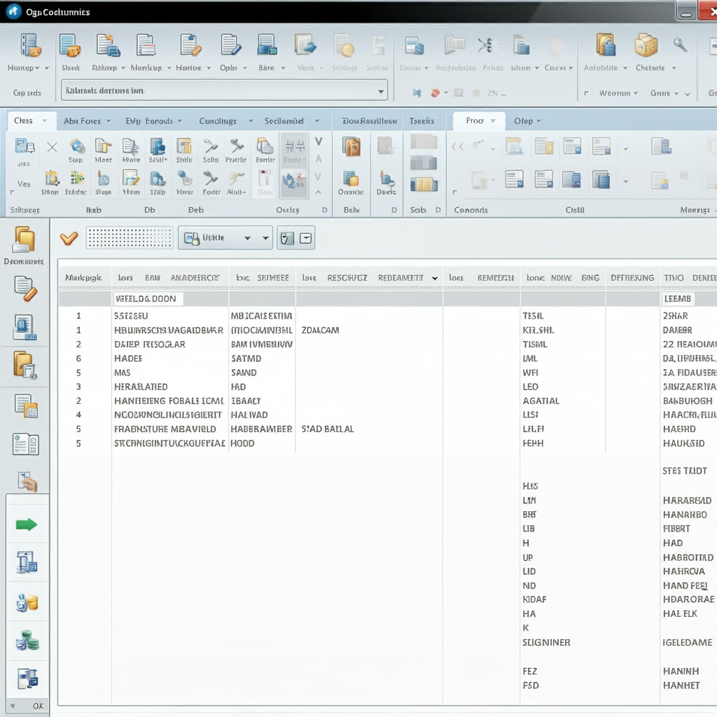
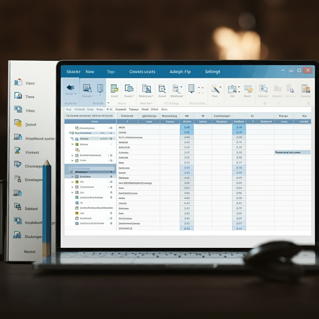
For instance, if you’re working with sales data, your header row might include titles such as Date, Product, Quantity Sold, and Revenue.
Suggested Image: A screenshot of an Excel spreadsheet showing a well-defined header row with relevant titles.
2. Creating a Header Row
To create a header row in Excel, follow these steps:
Step 1: Open Your Excel Spreadsheet
Start by launching Excel and opening the spreadsheet where you want to create a header row.
Step 2: Select the First Row
Click on the first row of your worksheet (Row 1) to select it. This is where you will input your header titles.
Step 3: Enter Your Header Titles
In each cell of the first row, type the appropriate title for each column. For example:
- A1: Date
- B1: Product
- C1: Quantity Sold
- D1: Revenue
Suggested Image: A screenshot showing the header titles being typed into the cells of the first row.
3. Formatting Your Header Row
Once you have entered your header titles, it’s important to format the header row to make it stand out.
Step 1: Select the Header Row
Highlight the entire first row by clicking on the row number on the left side of the worksheet.
Step 2: Apply Bold Formatting
With the header row selected, go to the Home tab in the ribbon. Click on the Bold button (or press Ctrl + B) to make the text bold.
Step 3: Change the Background Color
To further distinguish the header row, change the background color:
- With the header row still selected, click on the Fill Color icon in the Home tab.
- Choose a color that contrasts with the text color.
Step 4: Center the Text
Centering the text in your header row improves its appearance:
- With the header row still selected, click the Center alignment button in the Home tab.
- You can also adjust the font size and color to enhance readability.
Suggested Image: A screenshot of the formatting options in the Home tab, highlighting the Bold, Fill Color, and Center buttons.
4. Freezing the Header Row
When working with large datasets, it’s useful to keep the header row visible while scrolling. You can freeze the header row by following these steps:
Step 1: Select the Row Below the Header
Click on the row number of the second row (Row 2). This tells Excel that you want to freeze everything above this row.
Step 2: Freeze Panes
- Go to the View tab in the ribbon.
- Click on Freeze Panes in the Window group.
- Select Freeze Panes from the drop-down menu.
This action will keep your header row visible as you scroll down through your data.
Suggested Image: A screenshot of the View tab, highlighting the Freeze Panes option.
5. Using Filters with Header Rows
Using filters on your header row allows for easier data manipulation and analysis. Here’s how to add filters:
Step 1: Select the Header Row
Highlight the first row where your headers are located.
Step 2: Enable Filters
- Go to the Data tab in the ribbon.
- Click on Filter. This will add drop-down arrows to each header cell.
Step 3: Use Filters
You can now click the drop-down arrows to sort or filter the data in each column, making data analysis straightforward and efficient.
Suggested Image: A screenshot of a filtered Excel table with drop-down arrows visible on the header row.
6. Best Practices for Header Rows
To ensure your header rows are effective, follow these best practices:
- Keep Titles Short and Descriptive: Use concise titles that clearly describe the data.
- Consistent Formatting: Maintain consistent font styles and sizes for all header rows in your spreadsheet.
- Use Colors Sparingly: While colors can enhance visibility, too many colors can be distracting. Choose a color scheme that is professional and easy to read.
Suggested Image: An infographic summarizing best practices for creating effective header rows in Excel.
Conclusion
Creating a header row in Excel is a fundamental step in organizing and managing your data efficiently. By following the steps outlined in this guide, you can create a clear and functional header row that enhances the readability of your spreadsheets. Additionally, using features like freezing panes and filters can significantly improve your data analysis capabilities. With these tools at your disposal, you will be better equipped to handle and present your data effectively in Excel.
