How to Lock a Row or Column in Excel on a Mac
Freezing rows or columns in Excel is an essential feature that keeps specific sections of your spreadsheet visible while you scroll through other data. This is particularly useful for spreadsheets with headers or key information that you want accessible at all times. This guide walks you through the steps of freezing rows, columns, or both in Excel for Mac, with detailed instructions and images for each method.
1. Open Your Excel File
Before you start, open the Excel file where you want to freeze rows or columns.
- Step 1: Locate your Excel file and double-click to open it in Excel for Mac.
- Step 2: Scroll through your spreadsheet to identify the row or column you want to freeze.
2. Freezing the Top Row in Excel for Mac
If you want to freeze the top row to keep it visible as you scroll down, Excel for Mac makes it easy with a single click.
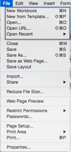
- Step 1: Open your spreadsheet and go to the View tab on the Excel toolbar.
- Step 2: In the View tab, find the Freeze Panes option.
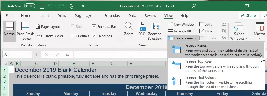
- Step 3: Click on Freeze Top Row. This option will freeze the top row so that it remains in place as you scroll through the rest of your data.
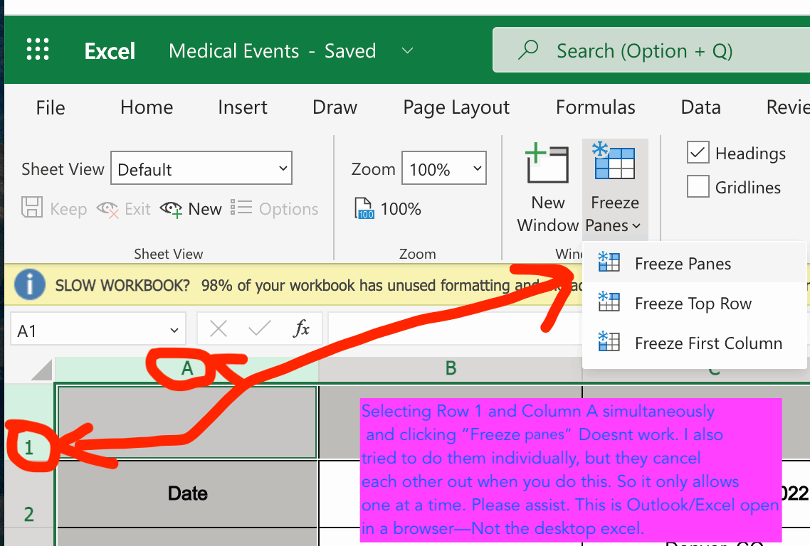
Once enabled, the top row will stay fixed at the top of your window even if you scroll down. This feature is especially useful if the top row contains headers that help identify each column’s data.
3. Freezing the First Column in Excel for Mac
Freezing the first column works similarly to freezing the top row. This can be helpful if the first column contains names or other identifiers that you want to see as you scroll across the sheet.
- Step 1: Go to the View tab on the Excel toolbar.
- Step 2: In the View menu, select Freeze First Column.

- Step 3: Now, the first column will remain in place as you scroll to the right.
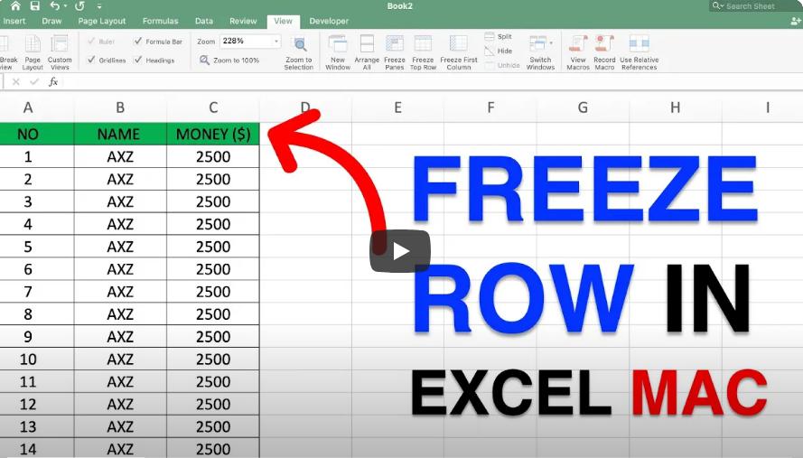
With the first column frozen, you’ll be able to reference its data as you move through other parts of your spreadsheet.
4. Freezing Multiple Rows or Columns in Excel for Mac
To freeze more than one row or column, you’ll need to use the Freeze Panes option, which lets you freeze multiple rows or columns above and to the left of a selected cell.
Steps for Freezing Multiple Rows
- Step 1: Select the row below the rows you want to freeze. For example, if you want to freeze the top three rows, click on the first cell in row 4.
- Step 2: Go to the View tab, click on Freeze Panes, and then choose Freeze Panes again from the dropdown.
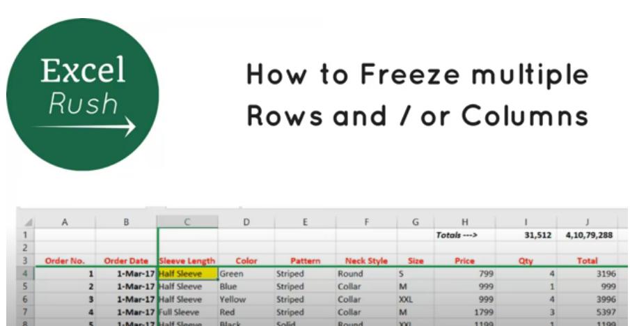
- Step 3: Excel will now freeze the specified rows, keeping them visible as you scroll down the sheet.
Steps for Freezing Multiple Columns
- Step 1: Select the column to the right of the columns you want to freeze. For example, if you want to freeze the first two columns, select the first cell in column C.
- Step 2: Go to the View tab, click on Freeze Panes, and choose Freeze Panes again.
- Step 3: The selected columns will stay in place as you scroll horizontally across your data.
5. Unfreezing Rows and Columns in Excel for Mac
If you decide that you no longer need certain rows or columns to be frozen, you can easily unfreeze them.
- Step 1: Go to the View tab in Excel.
- Step 2: Click on Freeze Panes and then select Unfreeze Panes from the dropdown menu.

All frozen rows and columns will return to their original scrollable state, allowing you to move through your spreadsheet freely.
Additional Tips for Freezing Panes in Excel for Mac
- Keyboard Shortcut: Unfortunately, Excel for Mac does not have a keyboard shortcut for freezing panes. However, you can quickly access this feature via the View tab.
- Ensure Active View: The Freeze Panes options are only available when your spreadsheet is in Normal view. If you’re in Page Layout or another view, switch back to Normal view under the View tab to enable freezing.
- Visible Borders: Frozen panes have a visible border at the edge of the frozen rows or columns, making it easy to distinguish the frozen section from the rest of the data.
Conclusion
Using the freeze feature in Excel for Mac can significantly enhance your workflow, especially when working with large datasets. By freezing rows and columns, you keep important headers or identifiers visible, making it easier to reference key information. With this guide, you should be able to freeze rows, columns, or both with ease, ensuring a smoother, more efficient experience in Excel.
