How to Insert Error Bars Representing Standard Deviation in Excel – 2024

How to Insert Error Bars Representing Standard Deviation in Excel

Adding standard deviation bars in Excel can be incredibly helpful for visualizing data variability and understanding the spread of your data around the mean. Standard deviation bars, also known as error bars, are useful in data analysis as they provide insights into how much the values in your dataset vary.

This guide will walk you through the steps to add standard deviation bars to your Excel charts with clear instructions and images.

Step 1: Set Up Your Data

First, you need to prepare your dataset in Excel. Ensure you have the values for which you want to add the standard deviation. The example below demonstrates how to calculate and add standard deviation bars to a sample dataset.

1. Enter Your Data: Enter your data in two columns, with labels for each category in the first column and the corresponding values in the second column.
   

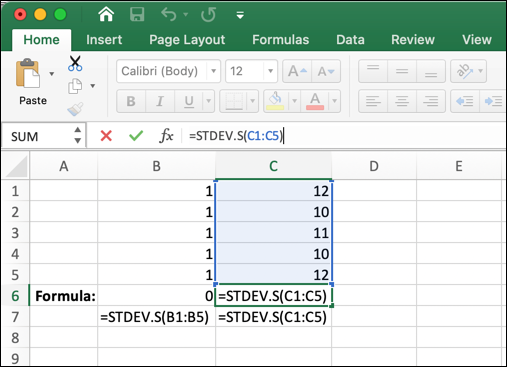
   Category	Value
   A	10
   B	15
   C	20
   D	25

2. Calculate Standard Deviation: If you want to display standard deviation bars based on calculated data, use the formula =STDEV.S(range), where “range” is the cell range of your values.

Step 2: Create Your Chart

Next, create a chart based on your data. A column chart is a popular choice for showing standard deviation bars.

1. Select the Data: Highlight your dataset (both the categories and the values).
2. Insert a Column Chart: Go to the Insert tab, select Insert Column or Bar Chart, and choose Clustered Column from the dropdown menu.

Your chart will appear with each category represented by a column.

Step 3: Add Error Bars to the Chart

To add standard deviation bars (error bars) to your chart:

1. Click on the Chart: Once your chart is created, click on it to select it.
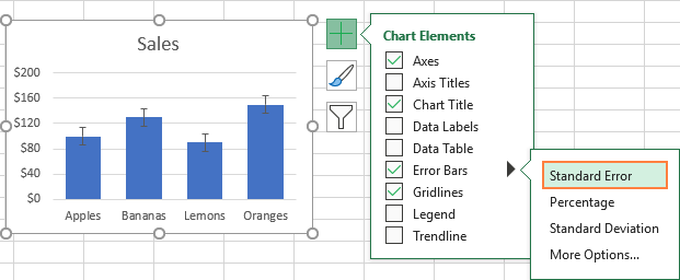
2. Go to the Chart Elements: Click on the + symbol next to the chart to open the Chart Elements menu.
3. Enable Error Bars: Check the box next to Error Bars.

This will add default error bars to your chart, but they may not yet reflect standard deviation.

Step 4: Customize Error Bars for Standard Deviation

Now that error bars are added, you need to adjust them to reflect the standard deviation values.

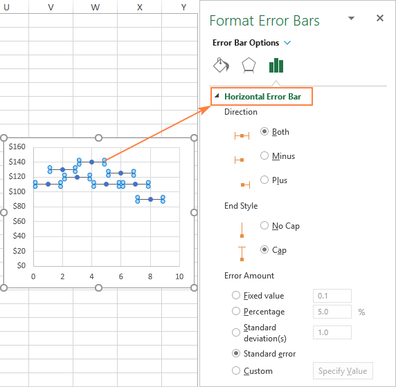
1. Open Error Bar Options: Click on one of the error bars on the chart. Excel will highlight all error bars, and a side pane will appear with options for customizing the error bars.
2. Select Custom: In the Format Error Bars pane, choose Custom under Error Amount. Then click Specify Value.
3. Enter Standard Deviation Values: In the dialog box that appears, enter the range for the standard deviation values you calculated in Step 1. Select the same range for both the Positive Error Value and Negative Error Value.

This will add standard deviation bars that represent the variability of each data point.

Step 5: Format the Error Bars (Optional)

You can adjust the appearance of the error bars to make them more noticeable:

1. Change Line Color: In the Format Error Bars pane, go to Line Color and choose a color that contrasts well with your chart.
2. Adjust Line Width: Increase the Width to make the error bars bolder if necessary.

Additional Tips

• Check Data Accuracy: Ensure that your standard deviation calculations are correct before adding error bars, as incorrect values will misrepresent your data.
• Use for Large Datasets: Standard deviation bars are particularly helpful when working with large datasets, as they provide a quick visual indication of data spread.
• Combine with Mean: To enhance data interpretation, consider adding a line representing the mean value.

By following these steps, you’ll be able to add standard deviation bars to your Excel charts quickly and accurately, helping you convey the variability of your data visually.