Excel Formatting Techniques: Functions, Conditional Formatting, Styles, and Beyond
Excel is a versatile tool that offers a wide range of formatting options to enhance the presentation and readability of data. Proper formatting not only improves the visual appeal of your spreadsheets but also makes data easier to interpret and analyze. This comprehensive guide will explore the various formatting functions, conditions, styles, and more, helping you master Excel formatting to make your data more effective and professional.
1. Understanding Excel Formatting Basics
Formatting in Excel involves changing the appearance of cells and their contents to improve clarity and presentation. Basic formatting includes adjusting fonts, colors, borders, and number formats.
Key Elements of Excel Formatting:
- Fonts and Colors: Change the font style, size, and color to make text more readable.
- Borders and Shading: Use borders and shading to separate sections and highlight important data.
- Number Formats: Format numbers as currency, percentages, dates, or custom formats for consistency and clarity.
Understanding these basic elements provides a foundation for more advanced formatting techniques.
2. Using Conditional Formatting in Excel
Conditional formatting in Excel allows you to apply formatting based on specific criteria, helping to highlight trends, identify outliers, and visually summarize data.
Step-by-Step Guide to Using Conditional Formatting:
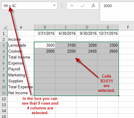
- Select Your Data Range:
- Highlight the cells you want to apply conditional formatting to.

- Go to the ‘Home’ Tab:
- Click on the “Home” tab on the Excel ribbon.

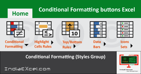
- Click on ‘Conditional Formatting’:
- In the “Styles” group, click “Conditional Formatting.”
- Choose a Rule Type:
- Select from options such as “Highlight Cells Rules,” “Top/Bottom Rules,” “Data Bars,” “Color Scales,” or “Icon Sets.”
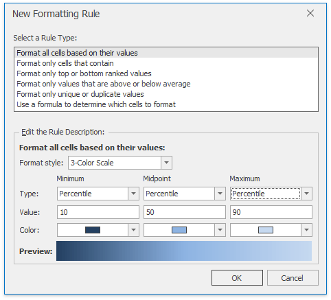
- Set Your Conditions:
- For example, to highlight cells greater than a certain value, select “Highlight Cells Rules” > “Greater Than…” and enter the value.

- Choose a Format:
- Select the formatting style (e.g., fill color, font color) to apply to cells that meet the criteria.

- Click ‘OK’ to Apply the Rule:
- Excel will apply the formatting based on your specified conditions.

3. Creating Custom Styles in Excel
Custom styles in Excel allow you to apply consistent formatting across your workbook, enhancing its visual coherence.
Step-by-Step Guide to Creating a Custom Style:
- Go to the ‘Home’ Tab:
- Click on the “Home” tab on the Excel ribbon.

- Click on ‘Cell Styles’:
- In the “Styles” group, click “Cell Styles.”

- Select ‘New Cell Style’:
- Choose “New Cell Style” from the dropdown menu.

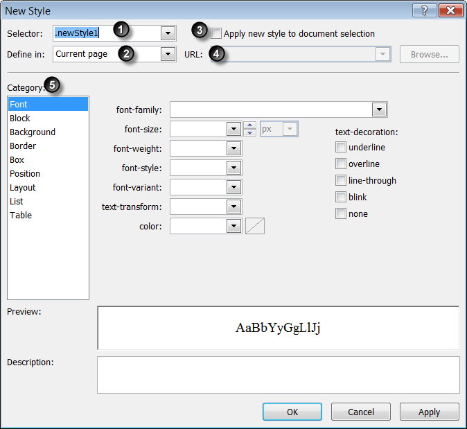
- Define Your Style:
- In the “Style” dialog box, enter a name for your style and click “Format” to define the formatting options (e.g., font, border, fill).
- Click ‘OK’ to Save Your Style:
- Once your style is defined, click “OK” to save it.
- Apply the Custom Style:
- To apply the style, select the cells you want to format, click “Cell Styles,” and choose your custom style.
4. Advanced Formatting Techniques: Using Functions for Dynamic Formatting
Excel functions like TEXT, DATE, and custom formulas can be used for dynamic formatting to display data in various formats automatically.
4.1 Using the TEXT Function for Formatting
The TEXT function allows you to format numbers and dates as text according to a specified format.
Example:
Convert a date to a specific format:
=TEXT(A1, “MM/DD/YYYY”)\text{=TEXT(A1, “MM/DD/YYYY”)}
Step-by-Step Guide:
- Enter the TEXT Formula:
- In the cell where you want the formatted result, enter the formula using the
TEXTfunction. 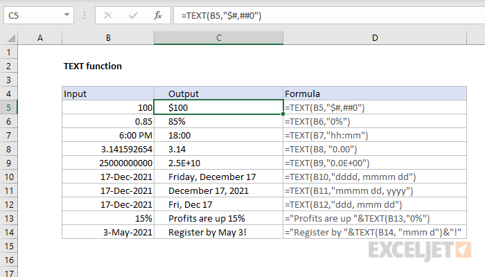
- In the cell where you want the formatted result, enter the formula using the
- Specify the Format:
- Define the format within quotes (e.g.,
"MM/DD/YYYY"for dates).
- Define the format within quotes (e.g.,
- Press Enter to Apply:
- Excel will display the formatted text in the specified format.
4.2 Using Custom Number Formats

Excel allows you to create custom number formats to display data according to your specific requirements.
Example:
Format a number with leading zeros:
=TEXT(A1, “00000”)\text{=TEXT(A1, “00000”)}
Step-by-Step Guide:
- Select the Cells to Format:
- Highlight the cells that you want to format.
- Open the Format Cells Dialog:
- Right-click the selected cells and choose “Format Cells,” or press
Ctrl + 1.
- Right-click the selected cells and choose “Format Cells,” or press
- Choose ‘Custom’ Under Number Tab:
- In the “Number” tab, select “Custom.”
- Enter Your Custom Format:
- In the “Type” field, enter your desired format (e.g.,
"00000"for numbers with leading zeros).
- In the “Type” field, enter your desired format (e.g.,
- Click ‘OK’ to Apply:
- Click “OK” to apply the custom number format.
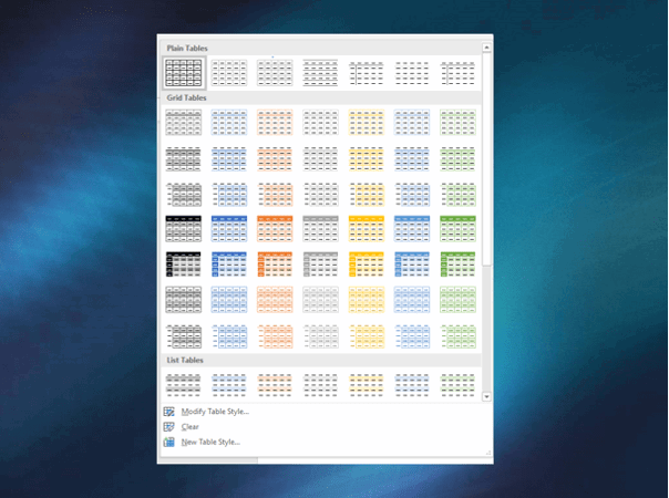
5. Applying Table Styles for Structured Data
Excel tables offer built-in styles that automatically format headers, rows, and columns, making your data more readable and visually appealing.
Step-by-Step Guide to Apply Table Styles:
- Select Your Data Range:
- Highlight the range of cells you want to convert into a table.

- Go to the ‘Insert’ Tab:
- Click on the “Insert” tab on the Excel ribbon.
- Click ‘Table’:
- Click the “Table” button in the “Tables” group.

- Choose a Table Style:
- Excel will automatically format your table with a default style, but you can change it by selecting “Table Styles” under the “Design” tab.
- Customize Table Style Options:
- You can further customize your table by selecting options like “Header Row,” “Total Row,” and “Banded Rows” in the “Design” tab.

- Click ‘OK’ to Confirm:
- Confirm your selections to apply the table formatting.
6. Best Practices for Excel Formatting
To maximize the effectiveness of your Excel formatting, consider these best practices:
- Keep it Simple: Avoid over-formatting; stick to a clean, consistent style that enhances readability.
- Use Conditional Formatting Sparingly: Too much conditional formatting can overwhelm users; use it to highlight key data points.
- Organize Data Effectively: Use tables and structured formats to keep data organized and easy to navigate.
- Leverage Built-in Styles: Use Excel’s built-in styles for quick, consistent formatting across your workbook.
Conclusion
Excel formatting is a powerful tool that goes beyond simply making your spreadsheet look good. By understanding and applying various formatting functions, conditions, and styles, you can enhance data readability, highlight important trends, and improve overall data presentation.
Whether you’re a beginner or an experienced Excel user, mastering formatting techniques can significantly improve your efficiency and effectiveness when working with data. Follow the steps outlined in this guide to enhance your Excel skills and make the most of this versatile tool. For more advanced formatting options, consider exploring Excel’s official resources or joining specialized training programs.

