Step-by-Step Guide to Creating a Drop-Down List in Excel
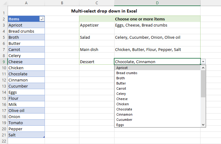
Adding a drop-down list in Excel can significantly enhance data entry by providing a predefined set of options for users to select from. This feature not only improves data consistency and accuracy but also makes your spreadsheets more interactive and user-friendly. In this comprehensive guide, we will walk you through the steps to create a drop-down list in Excel, complete with visual aids and examples.
1. Why Use a Drop Down List in Excel?
Drop-down lists in Excel are essential for several reasons:
- Improved Data Consistency: Ensures users select from a set of predefined options, reducing data entry errors.
- Enhanced User Experience: Makes spreadsheets more user-friendly and interactive.
- Streamlined Data Entry: Saves time by allowing users to select from a list instead of typing manually.
Understanding the benefits of drop-down lists can help you decide when and where to use them in your Excel workbooks.
2. Preparing Your Data for a Drop Down List
Before creating a drop-down list, it’s essential to prepare your data. Ensure that your list of options is organized in a single column or row in an Excel worksheet.
Example:

| A |
|---|
| Option 1 |
| Option 2 |
| Option 3 |
| Option 4 |
For instance, if you are creating a drop-down list for product categories, list all categories in a single column.
3. How to Add a Drop Down List in Excel
Excel provides a straightforward way to create drop-down lists using the Data Validation feature. Here’s a step-by-step guide to adding a drop-down list to your worksheet:
Step-by-Step Guide:
- Select the Cell for the Drop Down List:
- Click on the cell where you want to add the drop-down list.

- Go to the ‘Data’ Tab:
- Navigate to the “Data” tab on the Excel ribbon.

- Click on ‘Data Validation’:
- In the “Data Tools” group, click on “Data Validation.”

- Choose ‘List’ from the Allow Drop Down:
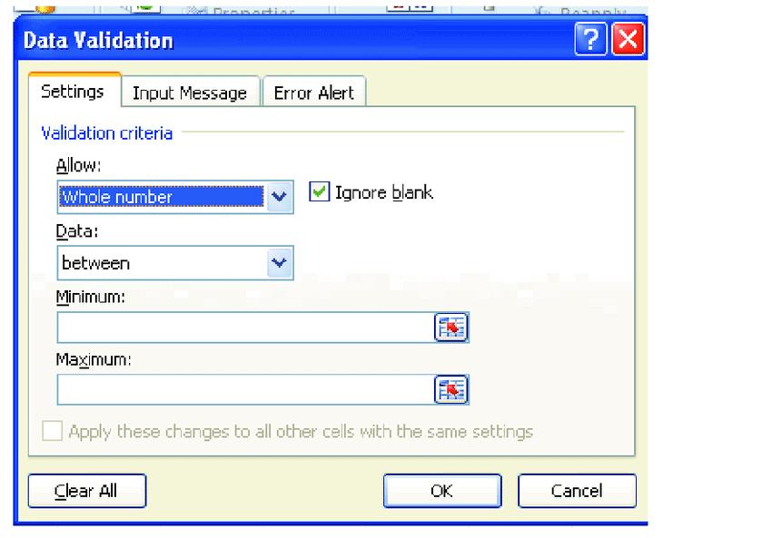
- In the Data Validation dialog box, select “List” from the “Allow” dropdown menu.

- Enter the Source Range:
- In the “Source” field, enter the range of cells containing the list options (e.g.,
=A1:A4), or type the list items directly separated by commas (e.g.,Option 1, Option 2, Option 3). 
- In the “Source” field, enter the range of cells containing the list options (e.g.,
- Click ‘OK’ to Create the Drop Down List:
- After entering the source, click “OK” to create the drop-down list.

- Test the Drop Down List:
- Click on the cell with the drop-down list to ensure it displays the list of options correctly.

4. Customizing Your Drop Down List
Excel allows you to customize your drop-down list further to enhance functionality and user experience.
4.1 Adding Input Message and Error Alerts
You can add an input message to guide users when they click on the drop-down list cell and set up an error alert to notify them when they enter invalid data.
Step-by-Step Guide:
- Go to ‘Data Validation’: Select the cell with the drop-down list and click “Data Validation” again.

- Set Up an Input Message:
- Click on the “Input Message” tab.
- Check “Show input message when cell is selected.”
- Enter a title and input message.

- Set Up an Error Alert:
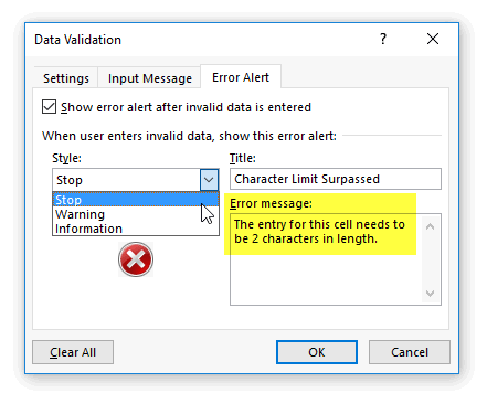
- Click on the “Error Alert” tab.
- Check “Show error alert after invalid data is entered.”
- Choose a Style (Stop, Warning, or Information), and enter a title and error message.

- Click ‘OK’ to Save Settings:
- Click “OK” to save the input message and error alert settings.

4.2 Allowing Users to Add New Items to the Drop Down List
To allow flexibility, you can let users add new items to the drop-down list.

Step-by-Step Guide:
- Go to ‘Data Validation’: Open the Data Validation dialog for the drop-down list cell.
- Uncheck ‘Ignore Blank’:
- Make sure the “Ignore blank” option is unchecked.
- Add New Items to the Source List:
- Simply add new items to the source list in the worksheet, and the drop-down list will automatically update.
5. Advanced Techniques: Creating Dependent Drop Down Lists
Dependent drop-down lists are lists that change based on the selection of another drop-down list. This is useful for hierarchical data, like selecting a country and then seeing cities in that country.
Step-by-Step Guide:
- Create the First Drop Down List: Follow the previous steps to create the main drop-down list (e.g., selecting a country).
- Define Named Ranges for Dependent Lists:
- Go to “Formulas” > “Define Name.”
- Create a named range for each dependent list (e.g., cities for each country).

- Create the Dependent Drop Down List:
- Select the cell for the dependent drop-down list.
- Go to “Data” > “Data Validation.”
- In the “Source” field, enter
=INDIRECT(A1)whereA1is the cell of the first drop-down list.

6. Best Practices for Using Drop Down Lists in Excel
To make the most out of drop-down lists in Excel, follow these best practices:
- Keep Lists Updated: Regularly update the source list to reflect the most current data.
- Use Named Ranges: For better manageability, use named ranges for list data.
- Limit the Number of Options: Keep the drop-down list concise to make it easier for users to select an option.
- Provide Clear Instructions: Use input messages and error alerts to guide users effectively.
Conclusion
Adding a drop-down list in Excel is a powerful way to enhance data entry and ensure consistency across your spreadsheets. By following the step-by-step guide and exploring advanced techniques, you can create dynamic, interactive, and user-friendly Excel sheets that improve efficiency and data accuracy.
Whether you’re using drop-down lists for simple data entry or more complex dependent selections, Excel’s data validation tools provide the flexibility and control needed to manage your data effectively. Regular practice and attention to detail will help you master this feature, making you more proficient in Excel. For further learning, consider exploring Excel’s official resources or joining Excel training programs.

