How to Compare Lists in Excel and Identify Differences
Comparing lists in Excel is a common task, whether you’re working with inventory data, customer records, or any other set of information. Finding the differences between two lists helps ensure data accuracy and can reveal missing or incorrect information. Fortunately, Excel provides several built-in functions and methods to help you quickly and efficiently compare lists.
In this guide, we will explore different ways to compare two lists in Excel, with detailed, step-by-step instructions and screenshots to guide you through the process.
Why Compare Lists in Excel?
There are many reasons why you may want to compare lists in Excel:
- Data Validation: Ensure two datasets are aligned and no values are missing.
- Inventory Management: Compare current stock lists against past records to identify discrepancies.
- Customer Information: Match and compare customer lists for updates or changes.
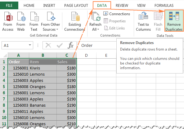
- Duplicate Entries: Remove duplicates or find unmatched values between two lists.
Method 1: Use Conditional Formatting to Compare Lists
One of the quickest and easiest ways to compare lists is to use Excel’s Conditional Formatting feature. This highlights differences between two lists visually.
Steps to Compare Lists Using Conditional Formatting
- Enter Your Lists in Excel:
- Suppose you have two lists in columns A and B.
- Select the First List:
- Highlight the values in column A (the first list).

- Apply Conditional Formatting:
- Go to the Home tab and click Conditional Formatting.
- Select Highlight Cells Rules > Duplicate Values.

- Choose Unique Values:
- In the Duplicate Values dialog box, select Unique from the dropdown menu.
- Choose a color format to highlight the differences and click OK.

- Review the Results:
- The unique values (those present in column A but not in column B) will be highlighted, allowing you to easily spot the differences.

Method 2: Compare Lists Using the IF Function
Another effective method is using the IF function, which allows you to compare two lists and display whether values match or differ.
Steps to Compare Lists Using IF Function
- Enter Your Lists in Excel:
- Assume you have two lists in columns A and B.
- Insert the IF Formula:
- In column C, enter the following formula in cell C2 to compare the lists:
excel=IF(A2=B2, "Match", "Different")
- This formula checks if the values in cells A2 and B2 are equal. If they are, it returns “Match”; if not, it returns “Different”.
- Drag the Formula Down:
- Copy the formula down for all the rows in column C to compare each corresponding value in columns A and B.
- Review the Results:
- The IF function will display “Match” if the values are the same and “Different” if they are not, making it easy to spot differences between the lists.
Method 3: Compare Lists Using the VLOOKUP Function
The VLOOKUP function is great for finding values in one list that don’t exist in the other.
Steps to Compare Lists Using VLOOKUP
- Enter Your Lists in Excel:
- For this example, let’s assume you have one list in column A and another in column B.
- Insert the VLOOKUP Formula:
- In cell C2, enter the following formula to check if values in column A exist in column B:
excel=IF(ISNA(VLOOKUP(A2, B:B, 1, FALSE)), "Not Found", "Found")
- This formula uses VLOOKUP to search for the value in cell A2 within column B. If it’s not found, the ISNA function will return “Not Found”; otherwise, it will return “Found”.
- Drag the Formula Down:
- Copy the formula down to compare all the values in column A with column B.
- Review the Results:
- You’ll see “Found” next to items that exist in both lists and “Not Found” next to those that do not.
Method 4: Compare Lists Using COUNTIF Function
The COUNTIF function is another versatile tool that can help you find differences between two lists by counting how many times each value appears in the second list.
Steps to Compare Lists Using COUNTIF
- Enter Your Lists in Excel:
- Place your lists in columns A and B.
- Insert the COUNTIF Formula:
- In cell C2, enter the following formula to compare the lists:
excel=IF(COUNTIF(B:B, A2)=0, "Not Found", "Found")
- This formula checks how many times the value in A2 appears in column B. If the result is zero, it returns “Not Found”; otherwise, it returns “Found”.
- Drag the Formula Down:
- Copy the formula down to compare all the values in column A.
- Review the Results:
- The formula will indicate which items in list A are missing from list B by returning “Not Found”.
Conclusion
Excel offers multiple methods for comparing lists, each suitable for different types of analysis. Whether you prefer using Conditional Formatting for a visual comparison, IF and VLOOKUP functions for a detailed check, or the COUNTIF function for counting occurrences, these tools can help you efficiently find differences between two lists.
By following the step-by-step instructions in this guide, you’ll be able to quickly spot discrepancies, ensuring your data is accurate and reliable. Whether you’re comparing customer lists, inventory data, or any other information, Excel makes it easy to find and address differences.
