Step-by-Step Guide: How to Build a Drop-Down List in Excel – 2024

Step-by-Step Guide: How to Build a Drop-Down List in Excel

A drop-down list in Excel is a powerful feature that makes data entry more efficient, consistent, and error-free. It allows users to select from a predefined set of values rather than typing manually, which is especially useful in large spreadsheets or forms. In this guide, we’ll walk you through a step-by-step process to create a drop-down list in Excel, including advanced techniques to enhance your spreadsheets.

1. Why Use a Drop-Down List in Excel?

Drop-down lists improve the accuracy and consistency of data by limiting input to a predefined set of options. They are useful for:

• Preventing Data Entry Errors: By offering only valid choices, you reduce the likelihood of mistakes.
• Speeding Up Data Entry: Selecting from a list is faster than typing, especially for repetitive data entry tasks.
• Improving Data Organization: Structured input makes it easier to sort and analyze data.

Understanding these benefits will help you leverage the drop-down list feature to optimize your Excel workflow.

2. Creating a Basic Drop-Down List Using Data Validation

The most straightforward way to create a drop-down list is by using the Data Validation feature in Excel.

Step-by-Step Guide to Creating a Basic Drop-Down List:

1. Select the Cell or Range for the Drop-Down List:
   • Click on the cell where you want the drop-down list to appear. You can also select a range if you want the list in multiple cells.
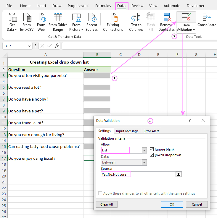
2. Go to the ‘Data’ Tab:
   • On the Excel ribbon, click on the “Data” tab.
3. Click on ‘Data Validation’:
   • In the “Data Tools” group, click on “Data Validation.”
4. Choose ‘List’ as the Validation Criteria:
   • In the Data Validation dialog box, go to the “Settings” tab. Under “Allow,” select “List.”
5. Enter the List of Options:
   • In the “Source” field, type the values you want to appear in the drop-down list, separated by commas. For example:

   $$Option1,Option2,Option3$$
6. Click ‘OK’ to Create the List:
   • After entering your list, click “OK.” The drop-down list will now appear in the selected cell or range.

3. Creating a Dynamic Drop-Down List from a Data Range

If you have a large list of items, it’s more efficient to create a dynamic drop-down list by referencing a data range in your worksheet.

Step-by-Step Guide to Creating a Drop-Down List from a Range:

1. Enter the List of Options in a Column:
   • Type your list of options in a column, such as A1

     . This will be the source of your drop-down list.
2. Select the Destination Cell for the Drop-Down List:
   • Click on the cell where you want the drop-down list to appear.
3. Go to ‘Data’ > ‘Data Validation’:
   • As before, go to the “Data” tab and click on “Data Validation.”
4. Select ‘List’ as the Validation Criteria:
   • In the Data Validation dialog box, select “List” under the “Allow” dropdown.
5. Enter the Range of Options in the Source Field:
   • In the “Source” field, enter the range of cells containing your list (e.g., =$A$1:$A$5).
6. Click ‘OK’ to Apply the Drop-Down List:
   • Click “OK,” and the drop-down list will be linked to your specified range.

4. Customizing the Drop-Down List with Input Messages and Error Alerts

You can make your drop-down list more user-friendly by adding input messages or error alerts that guide users when selecting options.

4.1 Adding an Input Message

An input message appears when a user clicks on the drop-down list, providing guidance or instructions.

Step-by-Step Guide to Adding an Input Message:

1. Select the Cell with the Drop-Down List:
   • Click on the cell where your drop-down list is located.
2. Open the ‘Data Validation’ Settings:
   • Go to “Data” > “Data Validation.”
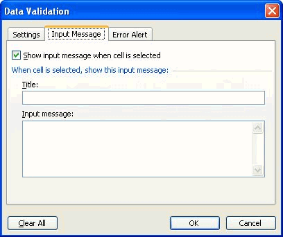
3. Click on the ‘Input Message’ Tab:
   • In the Data Validation dialog box, go to the “Input Message” tab.
4. Enter a Title and Message:
   • Enter a title and a brief message to display when the user clicks on the cell.
5. Click ‘OK’ to Save the Input Message:
   • Click “OK,” and the message will appear when the drop-down list is activated.

4.2 Setting an Error Alert

You can also set up an error alert to notify users when they attempt to enter invalid data.

Step-by-Step Guide to Adding an Error Alert:

1. Select the Drop-Down Cell:
   • Click on the cell containing the drop-down list.
2. Go to ‘Data Validation’:
   • Open the “Data Validation” dialog box again.
3. Select the ‘Error Alert’ Tab:
   • Click on the “Error Alert” tab.
4. Enter the Error Message:
   • Type in a title and an error message that will appear if the user enters invalid data.
5. Click ‘OK’ to Apply:
   • Click “OK” to save your error alert settings.

5. Best Practices for Using Drop-Down Lists in Excel

To ensure your drop-down lists work effectively, follow these best practices:

• Use Named Ranges for Large Lists: If your list of options is extensive, use a named range to simplify the process.
• Limit the Number of Options: Keep your list concise for ease of use.
• Use Conditional Formatting: Combine drop-down lists with conditional formatting to highlight selected data or flag invalid entries.
• Regularly Update the List: Keep your list of options up to date, especially when referencing a data range.

Conclusion

Creating a drop-down list in Excel is a valuable skill that improves data accuracy and streamlines workflows. Whether you’re setting up a simple list for a form or creating dynamic data ranges, mastering this feature will make your Excel spreadsheets more efficient and user-friendly.

By following the steps outlined in this guide, you can easily create drop-down lists, customize them with input messages and error alerts, and enhance your data management capabilities. For more advanced Excel features and best practices, consider exploring additional resources or taking Excel training courses to further refine your skills.